Fleet Performance for Different Risk Configurations
1. Introduction & Overview
In the effort of testing the hypothesis of offering higher returns by introducing higher risk fleets to SummerFi Lazy protocol, and the scalability and sustainability of this proposed strategy, we have implemented simulations to estimate the performance of specific fleets with different risk configurations to help understand the relationship between the aggressiveness of parameter setups and real fleet performance. We will explore three scenarios, low, mid, and high, where the first one is computed with the actual model configuration used for low-risk fleets. We will also vary the initial deposit capital in the range from $10K to $1B to visualize how flooding capital into small markets would ultimately decrease performance due to lower utilization. For borrowing demand, we have established a Gaussian random process that simulates utilization variations, consequently impacting ARK’s APYs and capital being trapped.
Our simulations reveal that mid-risk parameters could equal high-risk configurations for smaller deposits (under $1M-$10M) probably due to diversification, while high-risk setups become slightly advantageous within the range of $10M-$100M, though performance for all configurations eventually falls below that of larger and less risky protocols as capital approaches $100M-$500M and beyond. Notably, our simulations of currently deployed fleets show that for USDC on Ethereum and Base, these existing low-risk configurations already outperform the proposed high-risk fleets at relatively low TVLs ($10M), suggesting the proposed fleets may be unnecessary for these assets.
2. Fleet Parameter Setup
We have three setups for each high-risk fleet proposed in the SummerFi forum discussion forum post, where we have added additional arks we consider could enter into this category. With the exception of Maple, since simulations were done before Maple Finance reply on the forum, the following are the ark parameters per fleet provided by our risk model that we are using in our simulation:
Fleet Ethereum ETH
Fleet Ethereum USDC
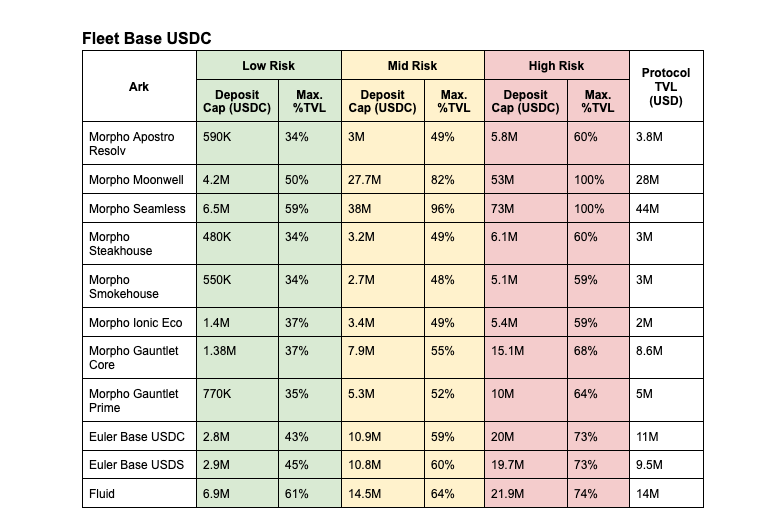
Fleet Base USDC
For the remaining parameters such as rebalance Inflow/Outflow, we have configured them so that Outflows allow the maximum cap to be withdrawn at once, while Inflows permit at most 20% of the total fleet cap to be deposited at once. We have left the fleet cap open (no cap) since we will vary the initial deposit during the simulation. Note that Fluid Protocol’s cap suggestions increase more slowly with risk due to its cooldown periods for withdrawals. We have also included the current TVL of each underlying protocol for comparison.
3. Borrowing Demand, Utilization, and Supply APY
In our simulation, we are going to simulate the keeper trying to chase the highest APY ark. Every time this happens, the total supply of the underlying protocol will change, and therefore the utilization, which impacts the final APY. Usually, the borrow rates are related to the utilization, which is the ratio between total borrows and total supply used as collateral. For simplicity, we will use,

and a generic curve for the borrow rates with the most common properties, i.e., a kink, a slow slope, and a high slope.
Fig. 1. Mock up of the Interest rate model used in the simulations.
Since each protocol has different parameters, we are going to set the slow slope using the current utilization and borrow rates on each protocol while fixing the base rates to 1%, kink to 85%, and high slope to 100%. Note that this is a mock-up model, since each lending protocol can have its own unique features when it comes to determining the borrow rates and the supply rates, e.g., Morpho has a time-dependent curve. Digging into the details of each protocol is out of the scope of this study. However, it is important to capture the basic effect of utilization, i.e., one gets higher borrow rates and higher supply APY at higher utilizations.
To simulate the borrow demand, we set a Gaussian random process that changes the utilization between 0 and 1. If the underlying protocol reaches utilization 1, it means the keeper is not able to withdraw the assets deposited there, although they will result in high APY. In general, if enough available liquidity is in the protocol and the keeper wishes to withdraw all the deposits, then it is allowed.
4. Simulation and Discussion
Every 6 hours, we set a new borrowing demand on each protocol, changing its APY, and for simplicity, the keeper is always able to withdraw (if enough liquidity is available) and deposit (without reaching the ark’s cap) consecutively into the highest APY arks, in order from highest to lowest until all capital of the fleet is used.
We will start with an initial fleet TVL that ranges between $10K - $1B, and simulate for a year tracking the total TVL after interest accrual. We will also analyze the influence of the final fleet APY as a function of the initial TVL, to study cases where markets have been overflooded with capital.
Fig. 2. Fleet Ethereum ETH. Performance as function of time and deposits for three scenarios, low, mid, and high risk parameters setup. The actual fleet currently deployed is denoted by Actual in the plot.
Fig. 3. Fleet Ethereum USDC. Performance as function of time and deposits for three scenarios, low, mid, and high risk parameters setup. The actual fleet currently deployed is denoted by Actual in the plot.
As we can see in Fig. 2, for fleet TVLs lower than $1M, the mid-risk setup performs equally as the riskiest one, suggesting that the extra risk is not worth taking based on the final performance. However, as we increase the initial TVL, at $100M, we can already see that the riskiest setup performs better than the middle one. Nevertheless, in the last plot, at around $500M in deposits, the Fleet APY is already lower than that provided by larger protocols such as AAVE, which could easily support $100M deposits with a less risky set of parameters, and where the current deployed fleet also starts outperforming the proposed configurations for all risk levels.
On the other hand, for the Fleet Ethereum USDC (Fig. 3.), we can observe that for low deposits, all risk configurations seem to deliver similar performance, and at $100M, the high-risk setup does it slightly better. However, having deposits as low as $10M, the current deployed fleet already starts outperforming this configuration for all risk levels, suggesting that the new fleet with the proposed arks may not be needed.
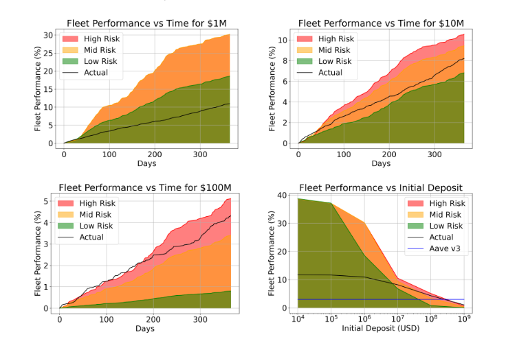
Fig. 4. Fleet Base USDC. Performance as function of time and deposits for three scenarios, low, mid, and high risk parameters setup. The actual fleet currently deployed is denoted by Actual in the plot.
Finally, for the case of the Fleet Base USDC, we can also see a similar tendency as for the Ethereum USDC, where with deposits at around $10M, the deployed fleet is already outperforming the proposed arks and fleet.
5. Conclusions & Remarks
We have studied the case of three fleets proposed in the SummerFi forum with three risk levels of parameter setups, also adding additional arks we consider could belong to this category. As the forum suggests, if the idea is to reach +$1B, we here show that the more capital is deposited into the fleets, the less effective APY we will get, resulting in most cases with the conclusion that having the assets in less risky and larger protocols, such as AAVE v3 or Sky, would be a better option. Therefore, while considering launching a “higher risk” fleets with the ARKs available in the tables above, we believe including the lower risk ARKs into those would increase the sustainability/scalability of those higher risk fleets (i.e. their APYs). In other words, the simulations show that having only “higher risk” ARKs in the higher risk fleets results in APY dilution as fleets TVL reaches some thresholds due to small pool sizes of those higher risk ARKs. If the proposed higher risk fleets were to have the lower risk ARKs with high TVL (e.g. Aave v3, Fluid, Sky, etc.), this threshold would be increased significantly.
Only for Ethereum ETH does the high-risk fleet show meaningful performance advantages, outperforming the current fleet until around $500M in deposits. For both USDC fleets (Ethereum and Base), our simulations reveal that the currently deployed fleets already outperform the proposed configurations at modest deposit levels of just $10M.
Also notice that double-digit performance at the fleet level consistently stops before reaching $100M in TVL. This is despite individual arks having double-digit APYs before considering the deposits of SummerFi.
Perhaps the results here suggest having, for the case of the fleet Ethereum ETH, a more aggressive fleet configuration and decreasing its risk profile as the TVL increases over time, while questioning the need for mid- and high-risk fleets for USDC on Base and Ethereum.